
व्याघ्र बीजगणित कॅल्क्युलेटर
सामान्य आणि मानक सामान्य वितरण
सामान्य वितरण
सामान्य वितरण (जी जीव्हाळणे, कौम्पाउन्ड-गौस्स, लाप्लेस–गौस्स वितरण, किंवा घंटारुप हेतु) ही संभाव्यतासंग्रहणाची वितरण वचनातील कोणत्याही अवर्णनशीलानुसार गणना अवर्णनशील या घालवी लागते. सामान्य वितरणाचे केंद्र सदैव मध्य मूल्यावर असते, जेथे वितरण संपूर्णतः समरूपी असते.
संकेतने
सांख्यिकीविदांनी सामान्यतः मोठी अक्षरे विपरीत घटकांचे प्रतिनिधित्व करण्यासाठी व लहान अक्षरे त्यांच्या मूल्यांचे प्रतिनिधित्व करण्यासाठी वापरतात. उदाहरणार्थ :
इतर उदाहरणे
: किती पेक्षा मोठी असेल त्याची संभाव्यता किती आहे?
: किती पेक्षा कमी असेल त्याची संभाव्यता किती आहे?
: आणि मधील असेल त्याची संभाव्यता किती आहे?
: पेक्षा मोठी आणि पेक्षा कमी असेल त्याची संभाव्यता किती आहे?
सामान्य वितरणाचे मापदंड
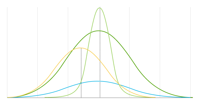
मध्य मूल्य व मानक विचलन हे सामान्य वितरणाचे दोन प्रमुख मापदंड आहेत. ते वितरणाच्या आकार आणि संभाव्यतांची निर्धारणे करतात.
मध्य
किंवा
The mean is the location of a distribution's center and peak, meaning any changes to the mean move the distribution curve to the left or right along the x-axis. Most data points (values) are located around the mean.
मानक विचलन
किंवा
मानक विचलन मूळ्यांच्या फरकांचा मोजमाप करते. ती साधारण वितरणाची अवधी निर्धारित करते. मोठे मानक विचलन यांमुळे होते, लहान विचलन यांमुळे होतात. लहान विचलन यांमुळे होतात.
सामान्य वितरणाची मालमत्ते
मानकीभूत सामान्य वितरण
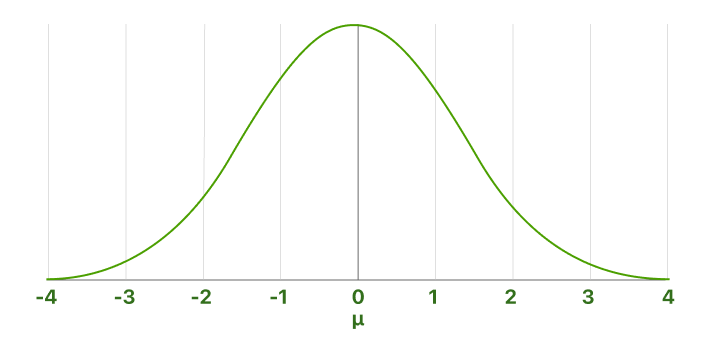
The standard normal distribution is a special case of the normal distribution in which the mean is zero and the standard deviation is one. This distribution is also referred to as a Z-distribution.
संकेतने
मानकीभूत स्कोर
मानक उत्तरोपांतील मूल्येला मानक उत्तरोपांतील मोजमाप किंवा z-स्कोर म्हणतात. It illustrates how many standard deviations above or below the mean a specific observation falls.
उदाहरणार्थ, a standard score of indicates that the observation is standard deviations above the mean. A negative standard score indicates a value below the average. The z-score of the mean is .
More than 99.9% of all results fall within +/- 3.9 standard deviations from the mean. Therefore, we regard the probability of data with a z-score greater than or less than as 0%. In other words, we consider the interval between and as 100% of the standard normal distribution.
Foil on the normal curve
The normal distribution is a probability distribution. As with any probability distribution, the proportion of the area that falls within two points on a graph of probability distribution indicates the probability that a value will fall within that range.
The total area under the curve equals , or 100% of the distribution. =100%.
When you get a z-score, you can find the area up to it by looking at a normal distribution table. It is also known as the z-scores table. (link to the table coming soon)
Since the z-score chart shows the area up to the z-score value, if you want to know the probability of data with greater z-scores, subtract the number from the table from . This rule can be expressed as:
If we don't find the perfect z-score in the table, we choose the closest one. If the two closest z-scores are equidistant from our desired z-score, we calculate their average.
Other examples
- What is the probability of data with a z-score that is larger than ?
- What is the probability of data with a z-score that is smaller than ?
- What is the probability of data with a z-score that is between and ?
- What is the probability of data with a z-score that is larger than and smaller than ?
मानकीकरण
z-स्कोर्स हे कसे गणतात
मानक स्कोर ही कोणत्याही निर्धारित जोखमाच्या मजबूत साहाय्यदायी असतात. त्या सामान्य वितरित लोकसंख्येतील वेगवेगळ्या मध्य व मानक विचलनवाल्या नियोजनातील लक्षणांची टाक करणारा मानकीत तयार करतात. मानकीकरणानंतर तुम्ही त्यांना मानक सामान्य वितरणामध्ये ठेवू शकता.
या प्रकारे, मानकीकरण आपल्याला प्रत्येक नियोजनमधील त्याच्या स्वतःच्या वितरणातील निर्धारित स्थानावर अध्वलीत असलेल्या वेगवेगळ्या प्रकारच्या नियोजनांची तुलना करण्याची संधी देते.
Take the raw measurement to compute the standard score for an observation, subtract the mean, and then divide by the standard deviation. Mathematically, the formula for that procedure is as follows:
refers to the raw value of the measurement we are interested in. It is the value to be standardized, often referred to as the data point.
(Mu) and (sigma) represent the parameters for the population from which the observation was drawn.
More related terms
स्विप्पण
The term "skewness" refers to a deviation or asymmetry that departs from the bell-shaped curve, or normal distribution, of a data set. If the curve shifts to the left or right, it is said to be skewed. Skewness can be quantified as a measure of the extent to which a particular distribution differs from a normal distribution. Skewness distinguishes between extreme values in one tail versus the other. A normal distribution has zero skewness.
कर्तिष
Kurtosis measures extreme values in either tail. Distributions with high kurtosis exhibit more extreme tail data than the tails of the normal distribution. Low kurtosis distributions display tail data that are generally less extreme than the tails of the normal distribution. Kurtosis is a measure of the combined weight of a distribution's tails relative to the center of the distribution. When a set of data that is nearly normal is graphed on a histogram, it appears as a bell curve, with most of the data within three standard deviations (plus or minus) of the mean. However, when there is a high level of kurtosis, the tails extend further than the three standard deviations of the normal bell curve distribution.
सामान्य वितरण (जी जीव्हाळणे, कौम्पाउन्ड-गौस्स, लाप्लेस–गौस्स वितरण, किंवा घंटारुप हेतु) ही संभाव्यतासंग्रहणाची वितरण वचनातील कोणत्याही अवर्णनशीलानुसार गणना अवर्णनशील या घालवी लागते. सामान्य वितरणाचे केंद्र सदैव मध्य मूल्यावर असते, जेथे वितरण संपूर्णतः समरूपी असते.
संकेतने
सांख्यिकीविदांनी सामान्यतः मोठी अक्षरे विपरीत घटकांचे प्रतिनिधित्व करण्यासाठी व लहान अक्षरे त्यांच्या मूल्यांचे प्रतिनिधित्व करण्यासाठी वापरतात. उदाहरणार्थ :
- ही गणना अवर्णनशील ची मूल्ये आहे.
- ही ची संभाव्यता दर्शविते.
- ही गणना अवर्णनशील विशेष मूल्य ला समान असण्याची संभाव्यता दर्शविते. उदाहरणार्थ, ही गणना अवर्णनशील मूल्य ला समान असण्याची संभाव्यता दर्शवते.
इतर उदाहरणे
: किती पेक्षा मोठी असेल त्याची संभाव्यता किती आहे?
: किती पेक्षा कमी असेल त्याची संभाव्यता किती आहे?
: आणि मधील असेल त्याची संभाव्यता किती आहे?
: पेक्षा मोठी आणि पेक्षा कमी असेल त्याची संभाव्यता किती आहे?
सामान्य वितरणाचे मापदंड
मध्य मूल्य व मानक विचलन हे सामान्य वितरणाचे दोन प्रमुख मापदंड आहेत. ते वितरणाच्या आकार आणि संभाव्यतांची निर्धारणे करतात.
मध्य
किंवा
The mean is the location of a distribution's center and peak, meaning any changes to the mean move the distribution curve to the left or right along the x-axis. Most data points (values) are located around the mean.
मानक विचलन
किंवा
मानक विचलन मूळ्यांच्या फरकांचा मोजमाप करते. ती साधारण वितरणाची अवधी निर्धारित करते. मोठे मानक विचलन यांमुळे होते, लहान विचलन यांमुळे होतात. लहान विचलन यांमुळे होतात.
सामान्य वितरणाची मालमत्ते
- ती समरूपी असते
सामान्य वितरणाची परिपूर्ण समरूपीता, अर्थात वितरणाचे वक्र मध्य मुळ्यावर, अर्थात मध्य मूल्यापासून दोन समान अर्धे तयार करण्यासाठी, मध्य मूल्यापासून दोन समान अर्धांची निर्मिती करण्यासाठी, वितरणाचे वक्र वळवी लागते. ही समरूपी आकृती एखाद्या आधीच्या निष्पत्तीचे परिणाम असते. - मध्य, मध्यीन आणि फारसाठवेली सर्व समान असतात
कारण सामान्य वितरण समरूपी असते, त्याच्या केंद्रावर सर्व डेटा बिंदूंचा सरासरी, किंवा मध्य मूल्य, असतो. ह्या म्हणजेच त्याच्या मध्य रेखापऱ्यंत किंवा मध्य मूळ म्हणजे त्याच्या केंद्राच्या गरीबेरीला असलेली केंद्री बांधली गेली होती आणि मध्य मूळ म्हणजे माहिती दर्शवितात. The peak, the tallest point of the normal distribution curve, also happens to be located at the center of the graph, meaning the distribution's mode, its most commonly occurring value and, therefore, the highest point on the graph, is also located at the distribution center. यातील येथे माहिती केंद्रोद्धर्ण दाखवते. The mean (average) is the point at which the most frequent occurrences occur. Accordingly, the midpoint (median) is also the point where these three measures fall. Such measures typically equate in a perfectly (normal) distribution. Half of the population is less than the center (mean) and half is greater than the center. - अनुभवी नियम
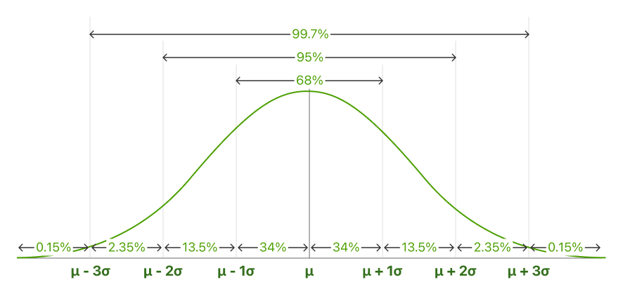
Also referred to as the 68-95-99.7 rule. The empirical rule describes the percentage of the data that fall within specific numbers of standard deviations from the mean for a bell-shaped curve.
Normally distributed data show a constant proportion of results within a given range of the mean. The Empirical Rule allows you to determine the proportion of values that fall within certain distances from the mean.
68.25% of all results fall within +/- one standard deviation from the mean.
95% of all results fall within +/- two standard deviations from the mean.
99.7% of all results fall within +/- three standard deviations from the mean.
मानकीभूत सामान्य वितरण
The standard normal distribution is a special case of the normal distribution in which the mean is zero and the standard deviation is one. This distribution is also referred to as a Z-distribution.
संकेतने
- ही "z-स्कोर" (मानक स्कोर) असते - z स्कोर म्हणजे किती मानक विचलन मूल्य मध्य मूल्यापासून आहे.
- (mu) ही मध्य मूल्य आहे.
- (sigma") ही मानक विचलन आहे.
मानकीभूत स्कोर
मानक उत्तरोपांतील मूल्येला मानक उत्तरोपांतील मोजमाप किंवा z-स्कोर म्हणतात. It illustrates how many standard deviations above or below the mean a specific observation falls.
उदाहरणार्थ, a standard score of indicates that the observation is standard deviations above the mean. A negative standard score indicates a value below the average. The z-score of the mean is .
More than 99.9% of all results fall within +/- 3.9 standard deviations from the mean. Therefore, we regard the probability of data with a z-score greater than or less than as 0%. In other words, we consider the interval between and as 100% of the standard normal distribution.
Foil on the normal curve
The normal distribution is a probability distribution. As with any probability distribution, the proportion of the area that falls within two points on a graph of probability distribution indicates the probability that a value will fall within that range.
The total area under the curve equals , or 100% of the distribution. =100%.
When you get a z-score, you can find the area up to it by looking at a normal distribution table. It is also known as the z-scores table. (link to the table coming soon)
Since the z-score chart shows the area up to the z-score value, if you want to know the probability of data with greater z-scores, subtract the number from the table from . This rule can be expressed as:
If we don't find the perfect z-score in the table, we choose the closest one. If the two closest z-scores are equidistant from our desired z-score, we calculate their average.
Other examples
- What is the probability of data with a z-score that is larger than ?
- What is the probability of data with a z-score that is smaller than ?
- What is the probability of data with a z-score that is between and ?
- What is the probability of data with a z-score that is larger than and smaller than ?
मानकीकरण
z-स्कोर्स हे कसे गणतात
मानक स्कोर ही कोणत्याही निर्धारित जोखमाच्या मजबूत साहाय्यदायी असतात. त्या सामान्य वितरित लोकसंख्येतील वेगवेगळ्या मध्य व मानक विचलनवाल्या नियोजनातील लक्षणांची टाक करणारा मानकीत तयार करतात. मानकीकरणानंतर तुम्ही त्यांना मानक सामान्य वितरणामध्ये ठेवू शकता.
या प्रकारे, मानकीकरण आपल्याला प्रत्येक नियोजनमधील त्याच्या स्वतःच्या वितरणातील निर्धारित स्थानावर अध्वलीत असलेल्या वेगवेगळ्या प्रकारच्या नियोजनांची तुलना करण्याची संधी देते.
Take the raw measurement to compute the standard score for an observation, subtract the mean, and then divide by the standard deviation. Mathematically, the formula for that procedure is as follows:
refers to the raw value of the measurement we are interested in. It is the value to be standardized, often referred to as the data point.
(Mu) and (sigma) represent the parameters for the population from which the observation was drawn.
More related terms
स्विप्पण
The term "skewness" refers to a deviation or asymmetry that departs from the bell-shaped curve, or normal distribution, of a data set. If the curve shifts to the left or right, it is said to be skewed. Skewness can be quantified as a measure of the extent to which a particular distribution differs from a normal distribution. Skewness distinguishes between extreme values in one tail versus the other. A normal distribution has zero skewness.
कर्तिष
Kurtosis measures extreme values in either tail. Distributions with high kurtosis exhibit more extreme tail data than the tails of the normal distribution. Low kurtosis distributions display tail data that are generally less extreme than the tails of the normal distribution. Kurtosis is a measure of the combined weight of a distribution's tails relative to the center of the distribution. When a set of data that is nearly normal is graphed on a histogram, it appears as a bell curve, with most of the data within three standard deviations (plus or minus) of the mean. However, when there is a high level of kurtosis, the tails extend further than the three standard deviations of the normal bell curve distribution.