
Tiger Algebra Calculator
Normal and standard normal distributions
Normal distribution
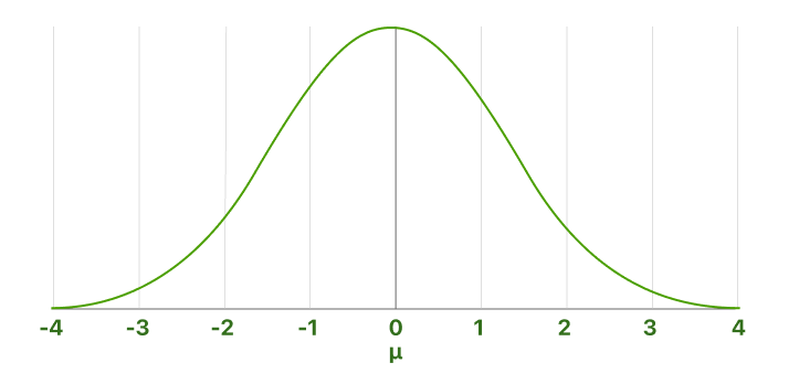
A normal distribution (also known as Gaussian, Gauss, or Laplace–Gauss distribution, or the bell curve) is a probability distribution that relates a cumulative probability with a random variable . The center of a normal distribution is always located at the mean, across which the distribution is completely symmetrical.
Notations
Statisticians typically use capital letters to represent random variables and lower-case letters to represent their values. For example:
Other examples
: What is the probability that is greater than ?
: What is the probability that is less than ?
: What is the probability that is between and ?
: What is the probability that is greater than and less than ?
Parameters of the normal distribution
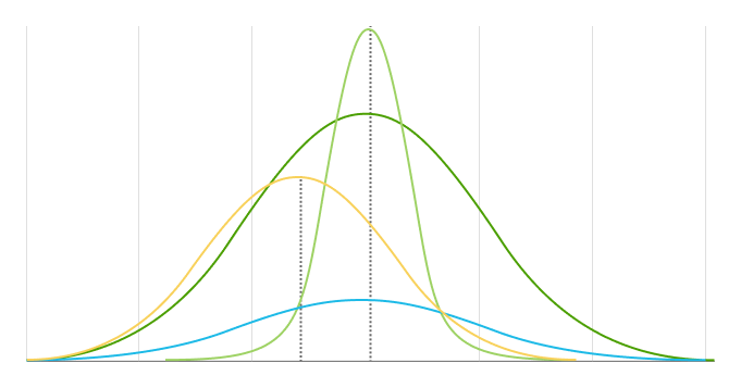
The mean and standard deviation are the two main parameters of a normal distribution. They determine both the distribution's shape and probabilities.
Mean
or
The mean is the location of a distribution's center and peak, meaning any changes to the mean move the distribution curve to the left or right along the x-axis. Most data points (values) are located around the mean.
Standard deviation
or
The standard deviation measures how far away data points are from a distribution's mean. It determines the width of a normal distribution. A larger standard deviation results in shorter, wider curves and smaller standard deviations results in taller, narrower curves.
Properties of the normal distribution
Standard normal distribution
The standard normal distribution is a special case of the normal distribution where the mean is zero and the standard deviation is one. This distribution is also called the Z-distribution.
Notations
Standard scores
A value on the standard normal distribution is called a standard score or a z-score. It represents the number of standard deviations above or below the mean that a specific observation falls.
For example, a standard score of indicates that the observation is standard deviations above the mean. A negative standard score represents a value below the average. The mean has a z-score of .
More than 99.9% of all cases fall within +/- 3.9 standard deviations from the mean. So, we regard the probability of any data with a z-score larger than or smaller than as 0%. In other words, we regard the interval between and as 100% of the standard normal distribution.
Finding areas under the curve of a standard normal distribution
The normal distribution is a probability distribution. As with any probability distribution, the proportion of the area that falls under the curve between two points on a probability distribution plot indicates the probability that a value will fall within that interval.
The area under the curve equals , and it's 100% of the distribution. =100%.
When you get a z-score, you can find the area up to it by looking at a standard normal distribution table. Also known as the z-scores table. (link to the table is coming soon)
Because the z-scores table shows the area up to the z-score value, when you want to find the probability of data with larger z-scores, you need to subtract the number from the table from . This can be shown as a rule:
When we don't find the perfect z-score in the table, we choose the closest one. If the 2 closest z-scores are the same distance from our wanted z-score, we calculate their mean.
Other examples
- What is the probability of data with a z-score that is larger than ?
- What is the probability of data with a z-score that is smaller than ?
- What is the probability of data with a z-score that is between and ?
- What is the probability of data with a z-score that is larger than and smaller than ?
Standardization
Calculating z-scores
Standard scores are a great way to understand where a specific observation falls relative to the entire normal distribution. They also allow you to take observations drawn from normally distributed populations with different means and standard deviations and place them on a standard scale. After standardizing your data, you can place them within the standard normal distribution.
In this manner, standardization allows you to compare different types of observations based on where each observation falls within its own distribution.
To calculate the standard score for an observation, take the raw measurement, subtract the mean, and divide by the standard deviation. Mathematically, the formula for that process is the following:
represents the raw value of the measurement of interest. It is the value to be standardized - sometimes called the data point.
(Mu) and (sigma) represent the parameters for the population from which the observation was drawn.
More related terms
Skewness
Skewness refers to a distortion or asymmetry that deviates from the symmetrical bell curve, or normal distribution, in a set of data. If the curve is shifted to the left or to the right, it is said to be skewed. Skewness can be quantified as a representation of the extent to which a given distribution varies from a normal distribution. Skewness differentiates extreme values in one versus the other tail. A normal distribution has a skew of zero.
Kurtosis
Kurtosis measures extreme values in either tail. Distributions with large kurtosis exhibit tail data exceeding the tails of the normal distribution. Distributions with low kurtosis exhibit tail data that are generally less extreme than the tails of the normal distribution. Kurtosis is a measure of the combined weight of a distribution's tails relative to the center of the distribution. When a set of approximately normal data is graphed via a histogram, it shows a bell peak and most data within three standard deviations (plus or minus) of the mean. However, when high kurtosis is present, the tails extend farther than the three standard deviations of the normal bell-curved distribution.
A normal distribution (also known as Gaussian, Gauss, or Laplace–Gauss distribution, or the bell curve) is a probability distribution that relates a cumulative probability with a random variable . The center of a normal distribution is always located at the mean, across which the distribution is completely symmetrical.
Notations
Statisticians typically use capital letters to represent random variables and lower-case letters to represent their values. For example:
- is the value of the random variable .
- represents the probability of .
- represents the probability that the random variable is equal to a particular value . For example, refers to the probability that the random variable is equal to .
Other examples
: What is the probability that is greater than ?
: What is the probability that is less than ?
: What is the probability that is between and ?
: What is the probability that is greater than and less than ?
Parameters of the normal distribution
The mean and standard deviation are the two main parameters of a normal distribution. They determine both the distribution's shape and probabilities.
Mean
or
The mean is the location of a distribution's center and peak, meaning any changes to the mean move the distribution curve to the left or right along the x-axis. Most data points (values) are located around the mean.
Standard deviation
or
The standard deviation measures how far away data points are from a distribution's mean. It determines the width of a normal distribution. A larger standard deviation results in shorter, wider curves and smaller standard deviations results in taller, narrower curves.
Properties of the normal distribution
- It is symmetrical
The normal distribution is perfectly symmetrical, meaning the distribution curve can be folded in the middle, along the mean, to produce two identical halves. This symmetric shape is the result of one-half of the observations falling on each side of the curve. - The mean, median, and mode are all equal
Because the normal distribution is symmetrical, its center represents the average, or mean, of all the data points. This means that its median (the value in the middle of a set when its values are ordered from least to greatest) is also located at the distribution center and is the same as the mean. The peak, the tallest point of the normal distribution curve, also happens to be located at the center of the graph, meaning the distribution's mode, its most commonly occurring value and, therefore, the highest point on the graph, is also located at the distribution center. These data of the normal distribution represent the data points (values) that occur. The mean is the center of the distribution because the mean is the point that occurs the most frequently. The midpoint is also the point where these three measures fall. The measures are usually equal in a perfectly (normal) distribution. Half of the population is less than the mean, and half is greater than the mean. - The empirical rule
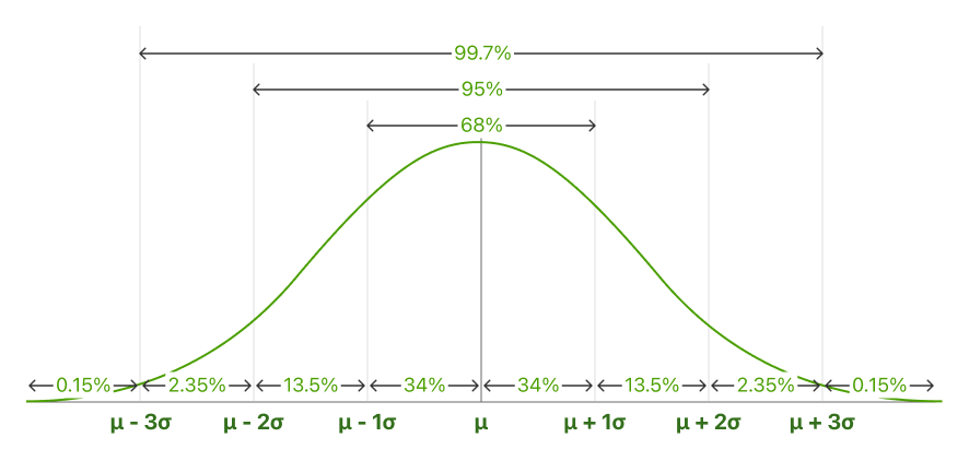
Also called the 68-95-99.7 rule. The empirical rule describes the percentage of the data that fall within specific numbers of standard deviations from the mean for bell-shaped curves.
In normally distributed data, there is a constant proportion of distance lying under the curve between the mean and a specific number of standard deviations from the mean. The Empirical Rule allows you to determine the proportion of values that fall within certain distances from the mean.
68.25% of all cases fall within +/- one standard deviation from the mean.
95% of all cases fall within +/- two standard deviations from the mean.
99.7% of all cases fall within +/- three standard deviations from the mean.
Standard normal distribution
The standard normal distribution is a special case of the normal distribution where the mean is zero and the standard deviation is one. This distribution is also called the Z-distribution.
Notations
- is the "z-score" (standard score) - z score is how many standard deviations a value is away from the mean.
- (mu) is the mean.
- (sigma") is the standard deviation.
Standard scores
A value on the standard normal distribution is called a standard score or a z-score. It represents the number of standard deviations above or below the mean that a specific observation falls.
For example, a standard score of indicates that the observation is standard deviations above the mean. A negative standard score represents a value below the average. The mean has a z-score of .
More than 99.9% of all cases fall within +/- 3.9 standard deviations from the mean. So, we regard the probability of any data with a z-score larger than or smaller than as 0%. In other words, we regard the interval between and as 100% of the standard normal distribution.
Finding areas under the curve of a standard normal distribution
The normal distribution is a probability distribution. As with any probability distribution, the proportion of the area that falls under the curve between two points on a probability distribution plot indicates the probability that a value will fall within that interval.
The area under the curve equals , and it's 100% of the distribution. =100%.
When you get a z-score, you can find the area up to it by looking at a standard normal distribution table. Also known as the z-scores table. (link to the table is coming soon)
Because the z-scores table shows the area up to the z-score value, when you want to find the probability of data with larger z-scores, you need to subtract the number from the table from . This can be shown as a rule:
When we don't find the perfect z-score in the table, we choose the closest one. If the 2 closest z-scores are the same distance from our wanted z-score, we calculate their mean.
Other examples
- What is the probability of data with a z-score that is larger than ?
- What is the probability of data with a z-score that is smaller than ?
- What is the probability of data with a z-score that is between and ?
- What is the probability of data with a z-score that is larger than and smaller than ?
Standardization
Calculating z-scores
Standard scores are a great way to understand where a specific observation falls relative to the entire normal distribution. They also allow you to take observations drawn from normally distributed populations with different means and standard deviations and place them on a standard scale. After standardizing your data, you can place them within the standard normal distribution.
In this manner, standardization allows you to compare different types of observations based on where each observation falls within its own distribution.
To calculate the standard score for an observation, take the raw measurement, subtract the mean, and divide by the standard deviation. Mathematically, the formula for that process is the following:
represents the raw value of the measurement of interest. It is the value to be standardized - sometimes called the data point.
(Mu) and (sigma) represent the parameters for the population from which the observation was drawn.
More related terms
Skewness
Skewness refers to a distortion or asymmetry that deviates from the symmetrical bell curve, or normal distribution, in a set of data. If the curve is shifted to the left or to the right, it is said to be skewed. Skewness can be quantified as a representation of the extent to which a given distribution varies from a normal distribution. Skewness differentiates extreme values in one versus the other tail. A normal distribution has a skew of zero.
Kurtosis
Kurtosis measures extreme values in either tail. Distributions with large kurtosis exhibit tail data exceeding the tails of the normal distribution. Distributions with low kurtosis exhibit tail data that are generally less extreme than the tails of the normal distribution. Kurtosis is a measure of the combined weight of a distribution's tails relative to the center of the distribution. When a set of approximately normal data is graphed via a histogram, it shows a bell peak and most data within three standard deviations (plus or minus) of the mean. However, when high kurtosis is present, the tails extend farther than the three standard deviations of the normal bell-curved distribution.